ODE-Solvers from Scratch
All the other tutorials show how to use the ODE-solver with the probsolve_ivp function. This is great, though probnum has more customisation to offer.
[1]:
from probnum import diffeq, filtsmooth, randvars, randprocs, problems
import numpy as np

import matplotlib.pyplot as plt

plt.style.use("../../probnum.mplstyle")
First we define the ODE problem. As always, we use Lotka-Volterra. Once the ODE functions are defined, they are gathered in an IVP object.
[2]:
def f(t, y):
    y1, y2 = y
    return np.array([0.5 * y1 - 0.05 * y1 * y2, -0.5 * y2 + 0.05 * y1 * y2])


def df(t, y):
    y1, y2 = y
    return np.array([[0.5 - 0.05 * y2, -0.05 * y1], [0.05 * y2, -0.5 + 0.05 * y1]])


t0 = 0.0
tmax = 20.0
y0 = np.array([20, 20])

ivp = problems.InitialValueProblem(t0=t0, tmax=tmax, y0=y0, f=f, df=df)
Next, we define a prior distribution and a measurement model. The former can be any Integrator, which currently restricts the choice to IBM, IOUP, and Matern. We usually recommend IBM. The measurement model requires a choice between EK0, EK1 (extended Kalman filters of order 0 or 1, respectively) and perhaps UK (unscented Kalman filter). The use of the latter is discouraged, because the square-root implementation is not available currently.
The measurement model can either be constructed with DiscreteEKFComponent.from_ode or, perhaps more conveniently, with GaussianIVPFilter.string_to_measurement_model.
[3]:
prior_process = randprocs.markov.integrator.IntegratedWienerProcess(
    initarg=ivp.t0,
    num_derivatives=4,
    wiener_process_dimension=ivp.dimension,
    forward_implementation="sqrt",
    backward_implementation="sqrt",
)
Next, we construct the ODE filter. One choice that has not been made yet is the initialisation strategy. The current default choice is to initialise by fitting the prior to a few steps of a Runge-Kutta solution.
[4]:
diffmodel = randprocs.markov.continuous.PiecewiseConstantDiffusion(t0=t0)
rk_init = diffeq.odefiltsmooth.initialization_routines.RungeKuttaInitialization()
ode_residual = diffeq.odefiltsmooth.information_operators.ODEResidual(4, ivp.dimension)
ek1 = diffeq.odefiltsmooth.approx_strategies.EK1()
firststep = diffeq.stepsize.propose_firststep(ivp)
steprule = diffeq.stepsize.AdaptiveSteps(firststep=firststep, atol=1e-3, rtol=1e-5)

solver = diffeq.odefiltsmooth.GaussianIVPFilter(
    steprule,
    prior_process=prior_process,
    information_operator=ode_residual,
    approx_strategy=ek1,
    initialization_routine=rk_init,
    diffusion_model=diffmodel,
    with_smoothing=True,
)
Now we can solve the ODE. To this end, define a StepRule, e.g. ConstantSteps or AdaptiveSteps. If you don’t know which firststep to use, the function propose_firststep makes an educated guess for you.
[5]:
odesol = solver.solve(ivp=ivp)
GaussianIVPFilter.solve returns an ODESolution object, which is sliceable and callable. The latter can be used to plot the solution on a uniform grid, even though the solution was computed on an adaptive grid. Be careful: the return values of __call__, etc., are always random variable-like objects. We decide to plot the mean.
[6]:
evalgrid = np.arange(ivp.t0, ivp.tmax, step=0.1)
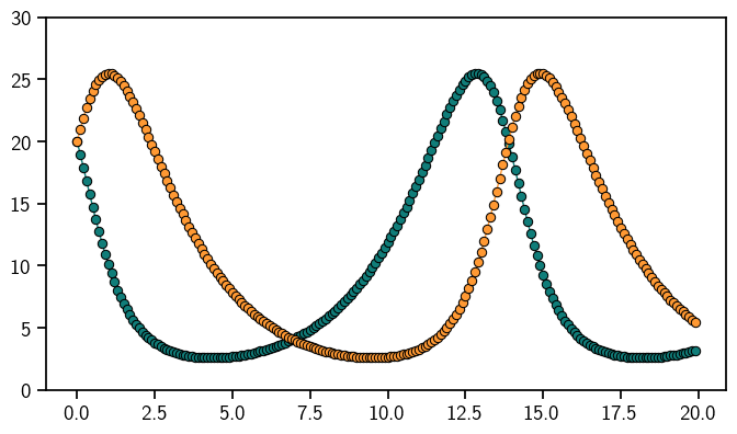
Done! This is the solution to the Lotka-Volterra model.
[7]:
sol = odesol(evalgrid)

plt.plot(evalgrid, sol.mean, "o-", linewidth=1)
plt.ylim((0, 30))
plt.show()
[ ]:
[ ]: